Automated Ball Shooter Simulator

Inspiration
Here is an article describing the automated ball shooter I worked on for my high school robotics team in 2020. From reading that you would know that it works by using a computer vision pipeline to find the target, calculate the distance between the robot and it, configure the shooting mechanism for it, and line the robot up.
But you may be wondering, how did we determine the correct flywheel RPM and hood angle for each distance? Originally, we were expecting to do some trial-and-error with the robot to get these values. However, the mechanical team ended up being a week behind schedule, and playing Counter Strike Source got rather boring, so we decided to make a Jupyter notebook that could simulate the physics of the ball being shot at various combinations of RPM and hood angles, choosing the best configuration for several distances from the target in 1-foot increments (4-24 feet).
How it Works
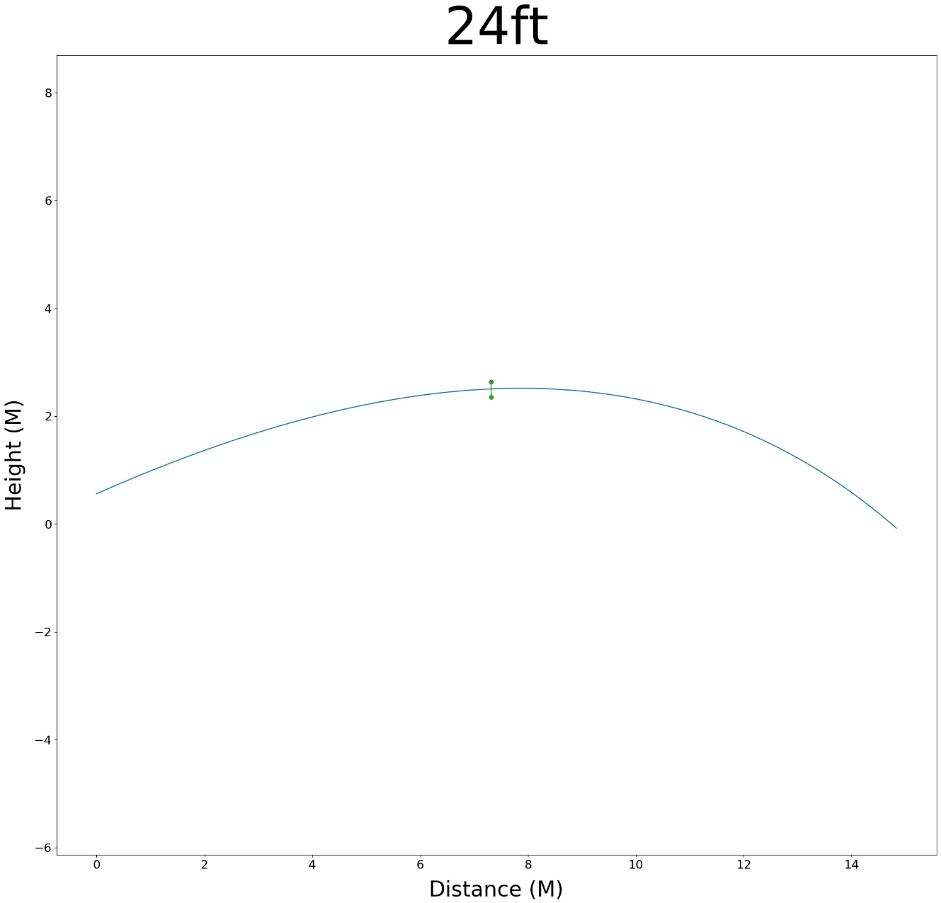
The simulation took a brute-force approach by going through and trying every possible combination of flywheel RPM and hood angle. For every combination, we were trying to minimize the vertical velocity of the ball as it goes through the center of the goal. For those of you familiar with projectile motion, this basically means we are trying to find the combination of flywheel RPM and hood angle such that the apex of the ball's trajectory ends up right in the center of the goal, as depicted in the image to the left below (the blue curve is the ball's trajectory, the small green vertical line is the entry of the goal):
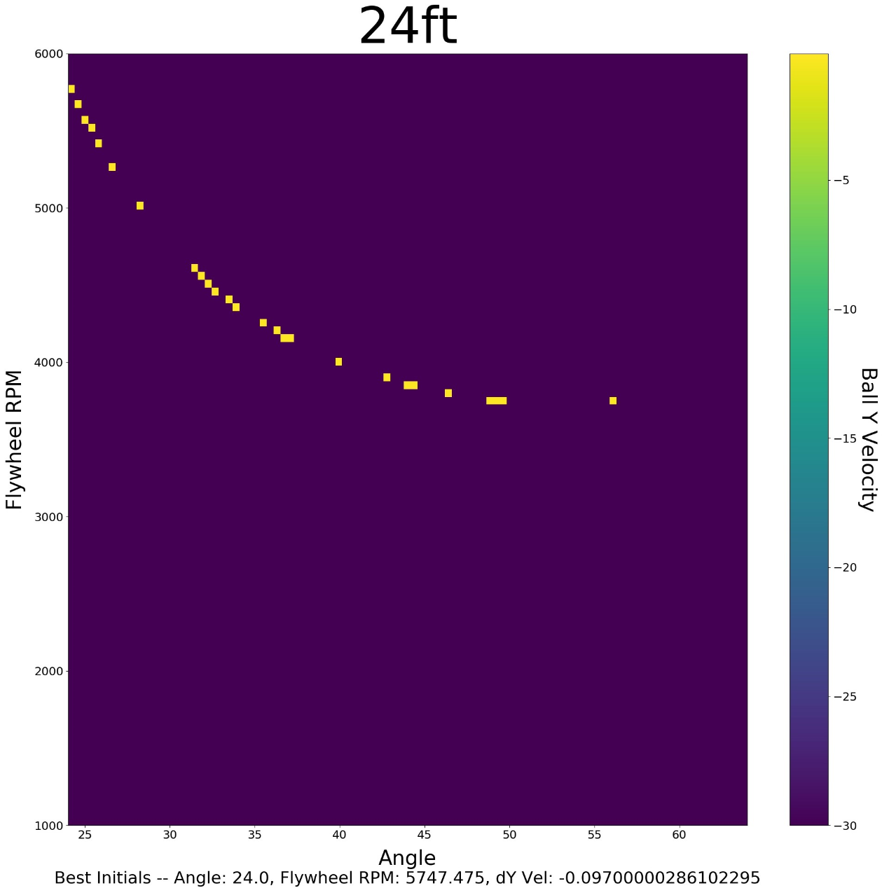
We also, for each distance, create a colormap as shown in the image to the right above. The horizontal axis is all of the possible hood angles, the vertical axis is the flywheel RPM. Then, to the right of the graph is a bar titled "Ball Y Velocity" (or the ball's vertical velocity) - this tells us how to interpret the colors in the actual colormap. So, yellow means the ball's vertical velocity going through goal was about 0 meters per second (m/s), and purple means the vertical velocity going through the goal was 30 m/s.
As you may have noticed, towards the bottom it tells us the best values. So you may ask, what is the purpose of the graph? The answer to which is that we can see how all the other combinations of flywheel RPM and hood position worked out, but also, they just look cool 😎.
My primary role was creating these visualizations to help us understand the data the simulation was giving.
Challenges
The biggest challenge was working out the physics of the ball. This took a lot of research (and a lot of interesting papers from NASA) to work out, but it was a fun learning process as we worked out the math on a whiteboard together. In the end, the predictions made by the simulator were actually pretty good, and only needed minor adjustment.
What I Learned
It was interesting to learn about "real world" projectile motion, where you need to account for things like drag coefficient of the projectile, its angular velocity, the density of the air, and the magnus effect on projectiles. It's a fun experience to apply things you've learned in the classroom to solve real problems.
See the Code
Here is the Jupyter notebook I worked on.