Custom FRC Pipelines
Inspiration
Majority of my work in my last 2 years on my FRC team involved computer vision. CV and its applications to robotics have always been very interesting to me. However, most of what ended up on our robot used a system called the Limelight. It's an all-in-one computer vision platform with a camera and small computer on board that runs the computer vision pipelines.
The Limelight was very nice, but it was expensive, and would sometimes randomly crash for no apparent reason. So, out of the desire to learn more about CV I set out to build my own alternative to the Limelight. While it never ended up being used on one of the robots, it worked rather well and I learned many new things working on it.
How the Pipeline Works
A pipeline is a sequence of distinct steps to process and analyze image data. It can be used to find how far away we are from an object or our orientation with respect to it. Here is an overview of how we go from an image to finding how far away we are from say, a goal marked with retroreflective tape.
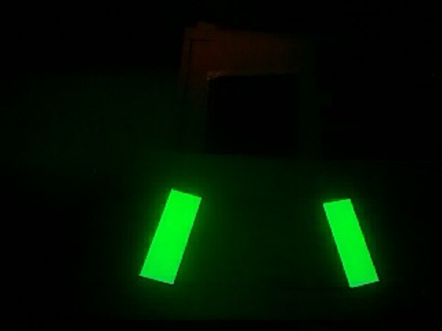
1) Capturing the Image
The first step is capturing a frame. We only care about the target (the retroreflective tape) within the frame, so we want to capture the frame in way that makes it stand out. To do this, we shine the target with a bright light, adjust the white balance to make it really stand out, and we bring the camera ISO and shutter speed down, removing (nearly) all unwanted pixels.
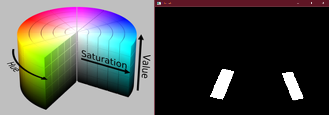
2) Thresholding
While we got rid of a most of the unwanted pixels, there are still some left over, which we can get rid of using thresholding. To do this, we convert the image into the HSV (Hue, Saturation, and Value) color space. Hue is "pure color", Saturation is how saturated the pure color is, and Value is the amount of black in a color (see the color cylinder below). We simply specify the ranges of Hue, Saturation and Value we want thresholding to keep. The result is a monospace image, where every pixel is either 1 (white) or 0 (black).
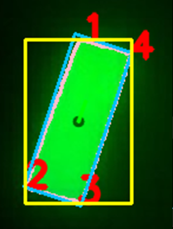
3) Contour Detection
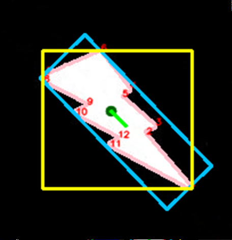
Next we can begin to look for objects - otherwise known as contours within the image. For each contour we calculate a few properties: The contour boundary (pink), the contour midpoint (dark green), the contour reference vector (green), the contour vertices (red), the contour area, the contours' Oriented Bounding Box or OBB (blue), and lastly the contours' Axis-Aligned Bounding Box or AABB (yellow).
4) Contour Filtering
Contour detection isn't a "smart" process, as in it won't pick up exactly what you want and only that - it will pick up any object of any shape and size. So, we can filter through the contours we found to get exactly what we want. We can filter by the contour area, fullness, which is the contour area divided by the area of the OBB, and lastly the aspect ratio of the AABB.
We then sort our filtered contours, either from left to right, right to left, top to bottom or bottom to top.
5) Contour Pairing
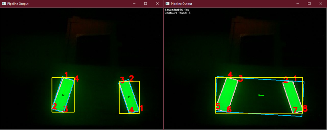
Sometimes, a target may consist of multiple contours, as is shown in the image below. In this case, we can perform contour pairing. The pairs are created from our list of filtered and sorted contours. Multiple pairs can be created, and we can filter and sort our pairs just as we did with the individual contours. We can also specify an intersection location for the contours - basically, if you were to draw a line through each contour, parallel to the reference vector, they would either intersect above, below, to the right or to the left of the contours, and we can specify this.
6) Choosing the Target
Now we choose our target. If we did not perform contour pairing, we chose the first contour in the list of filtered and sorted contours. Else, we choose the first contour pair in the list of filtered and sorted contour pairs. Whichever case, we now theoretically have the target closest to what the pipeline specifies, and we can now perform Pose Estimation.
7) Performing Pose Estimation
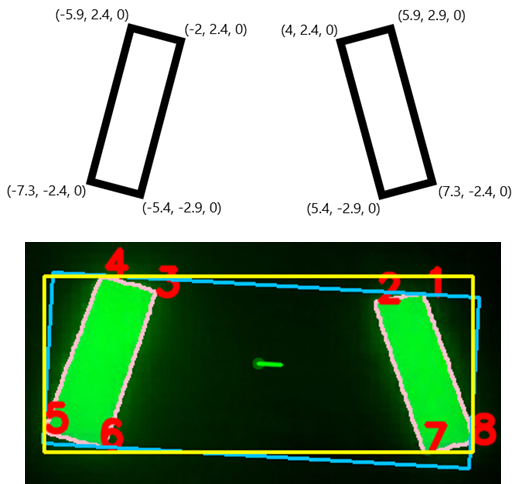
Pose Estimation is a process where we obtain the position and orientation of a 3D object from a 2D image, with respect to the camera sensor. This can be done with a simple OpenCV call, which takes a Camera Matrix, containing the intrinsic and extrinsic properties of the camera; the distortion coefficients of the camera; the objects points, or the location of the points of interest of the target in the real world; and the image points, which are the locations of the points of interest within the frame in pixel space.
We can then use this data to align ourselves with the target, or drive straight up to it, performing complex tasks and maneuvers that would originally have to have been manually by the driver in a matter of seconds.
The image to the right shows a targets image points marked in red, with its corresponding object points shown above (measured in inches).
Using Double Buffering to Improve Performance
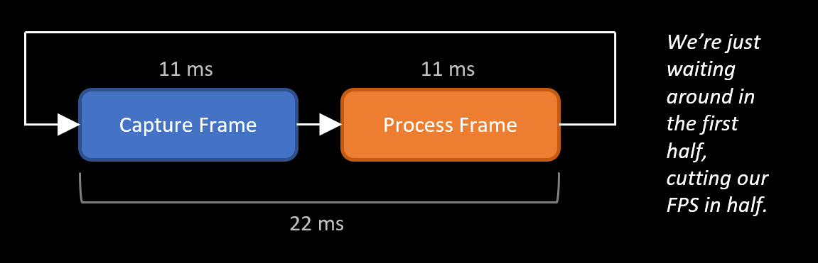
Now we have our pipeline, but how do we run it? At first you may just implement an infinite loop, where you grab a frame, run it through the pipeline, and repeat. There is an inherent issue with this, however. Say you want to run the pipeline at 90 FPS, which means we must spend no more than about 11 ms (milliseconds) processing each frame. Let's also say the pipeline takes 11 ms to run.
The camera will be running at 90 FPS so you can have a new frame every 11 ms. The issue here is, the process of capturing a frame isn't instantaneous - it takes time, which in this scenario is 11 ms. So, our current approach would take 22 ms to process each frame (halving the desired FPS), because we're spending half of the time sitting around, waiting for the frame to come. Here's a visual explaining the issue:
This can be solved using double buffering. There is a good explanation here on how it works conceptually. To implement this, we'll have two threads - a capture thread and a processing thread. The former has two buffers, and all it does it wait for a frame, store it in one of the buffers, swap the pointers to the buffers, wait for the next frame, and repeats the whole process. The latter, rather than waiting for a frame will simply grab the last one from the capture thread - so we are no longer waiting around for a frame. This is depicted in the image below:
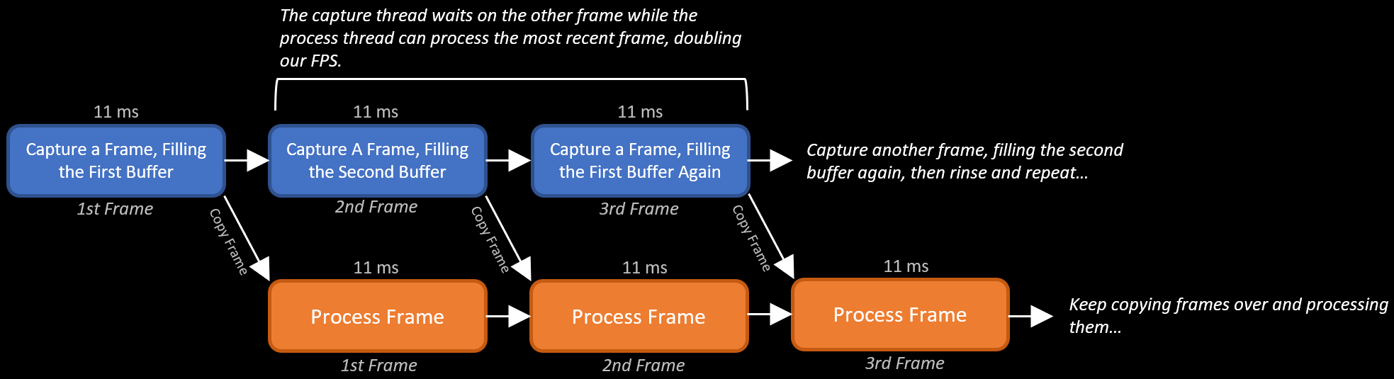
Similar to our original approach, the data when processed will still be 22 ms old, however, we have doubled our FPS, giving us double the data in the same amount of time.
The Hardware
As this was going to be on our robot, it needed some compact platform to run off of. I decided to use a Raspberry Pi, with a Raspberry Pi Camera and a some bright green LED's to make the targets easier to see. I decided to go with the Pi simply because it was cheap, compact, and still packing some good performance. I chose the Pi Camera because it was much more compact then a USB webcam, and it connects to the Pi via a CSI interface, which has much more bandwidth than USB.
This the first revision of the hardware, with the Pi, Pi Cam, an LED ring light, a VRM to help supply power to everything, and a 3D printed plate to hold it all together.
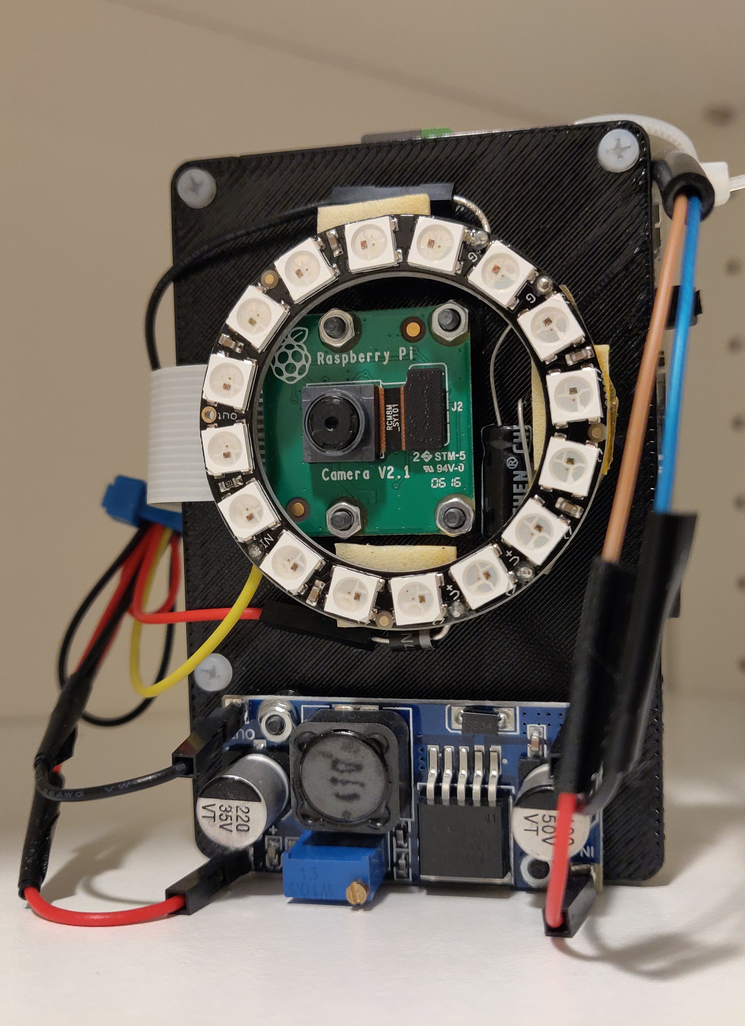
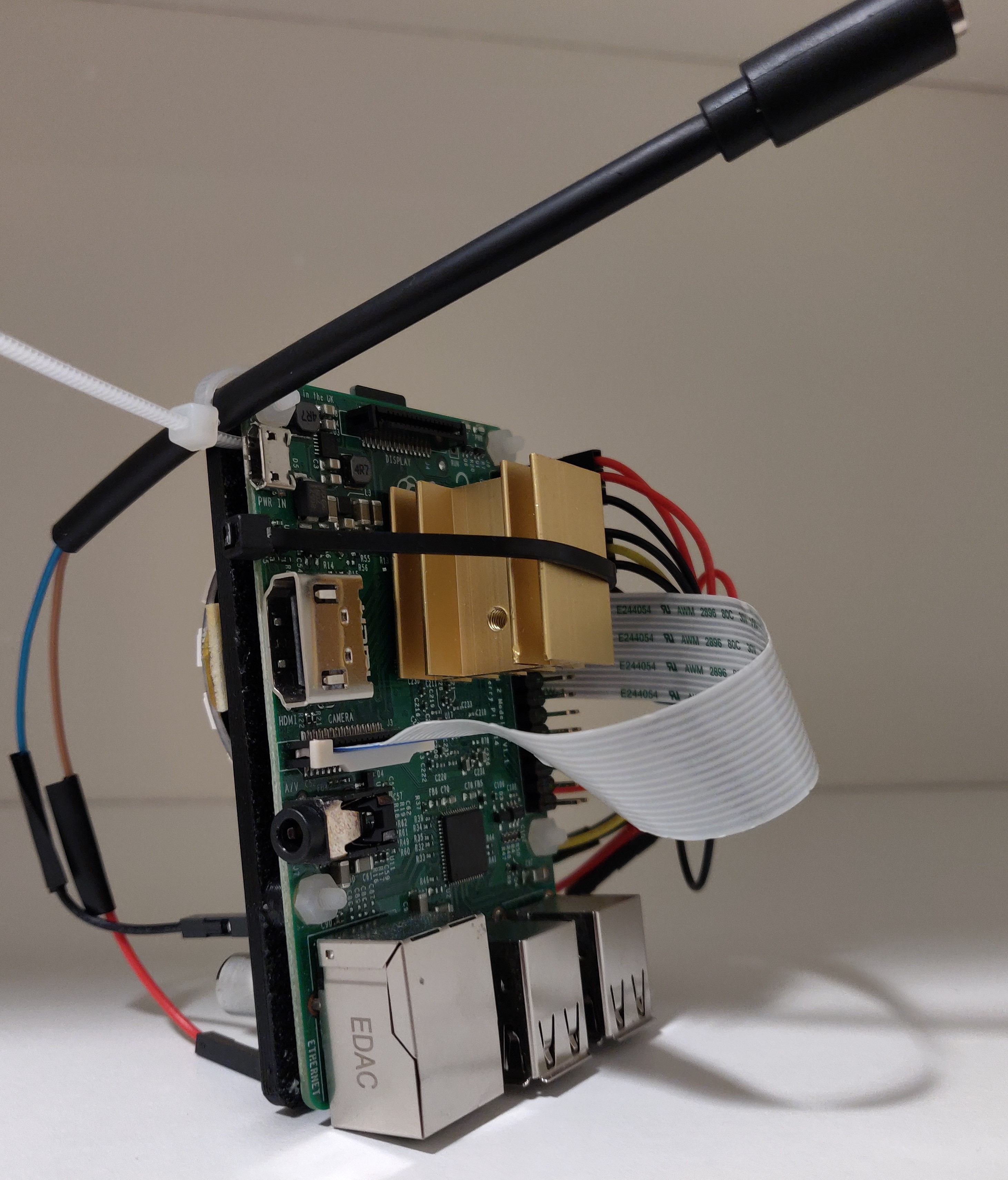
This was alright in the beginning, but it had its drawbacks. It was difficult to handle, the LED's weren't nearly as bright as they needed to be, and we still needed some more compute power. Enter the V2:
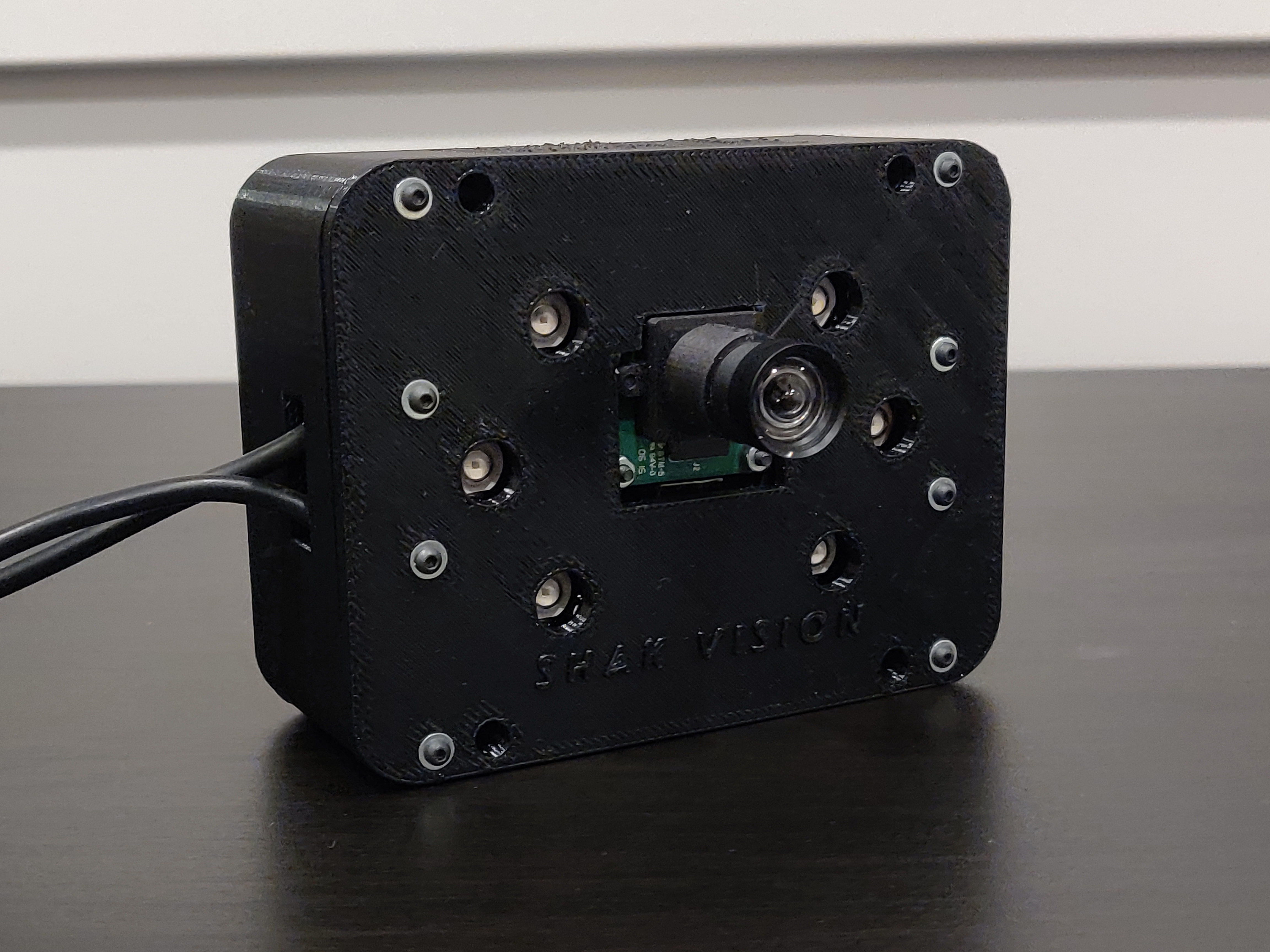
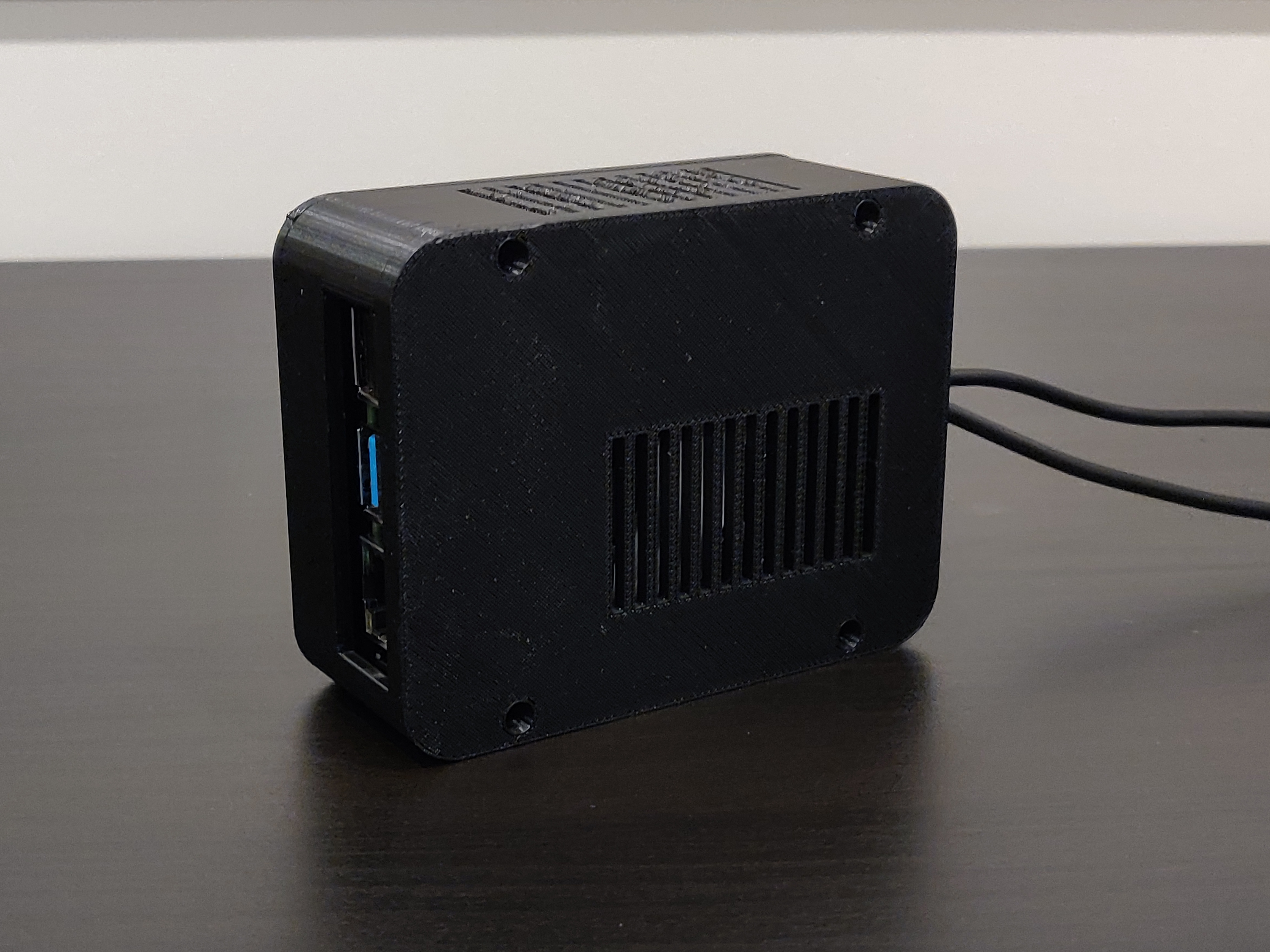
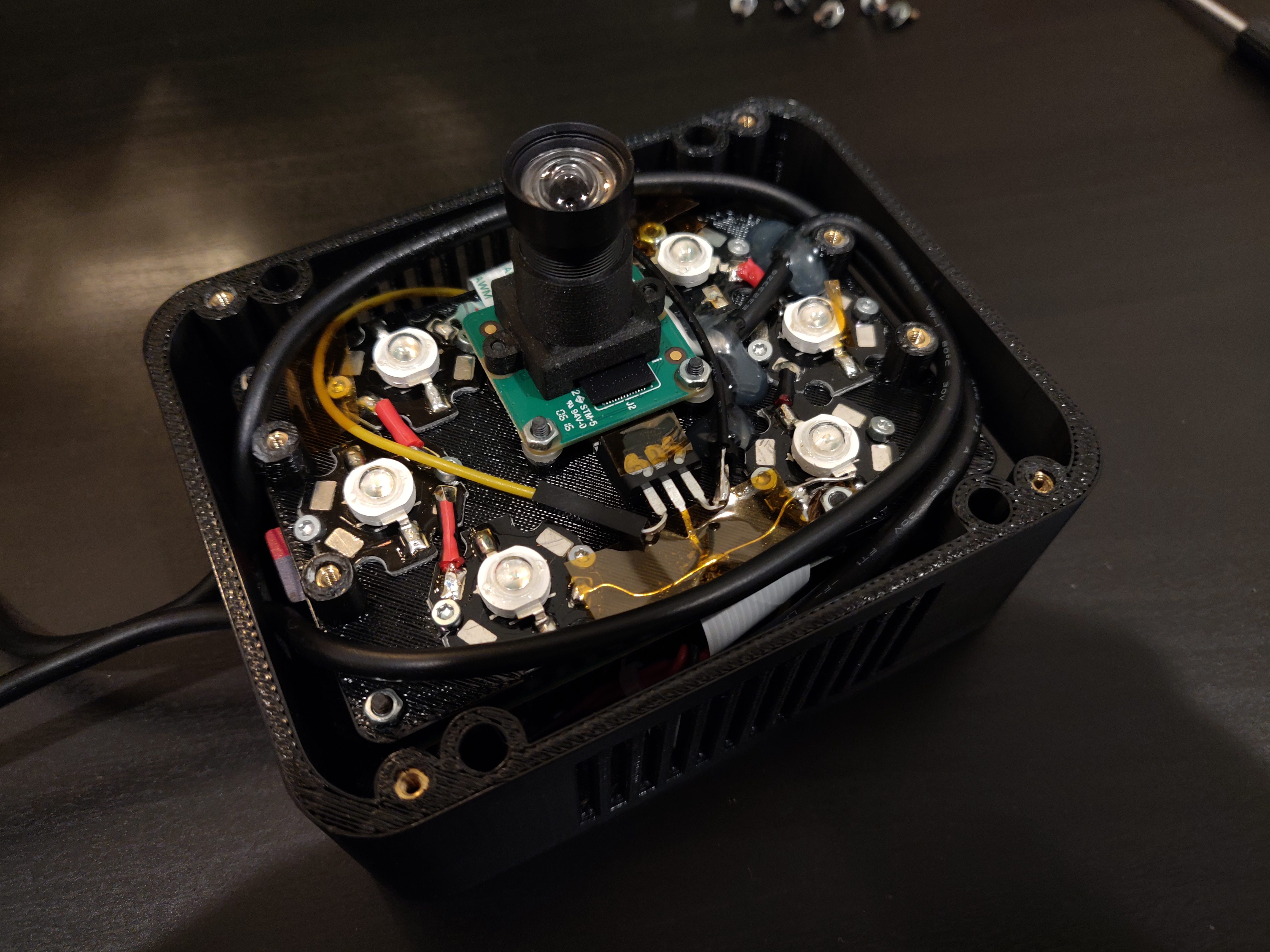
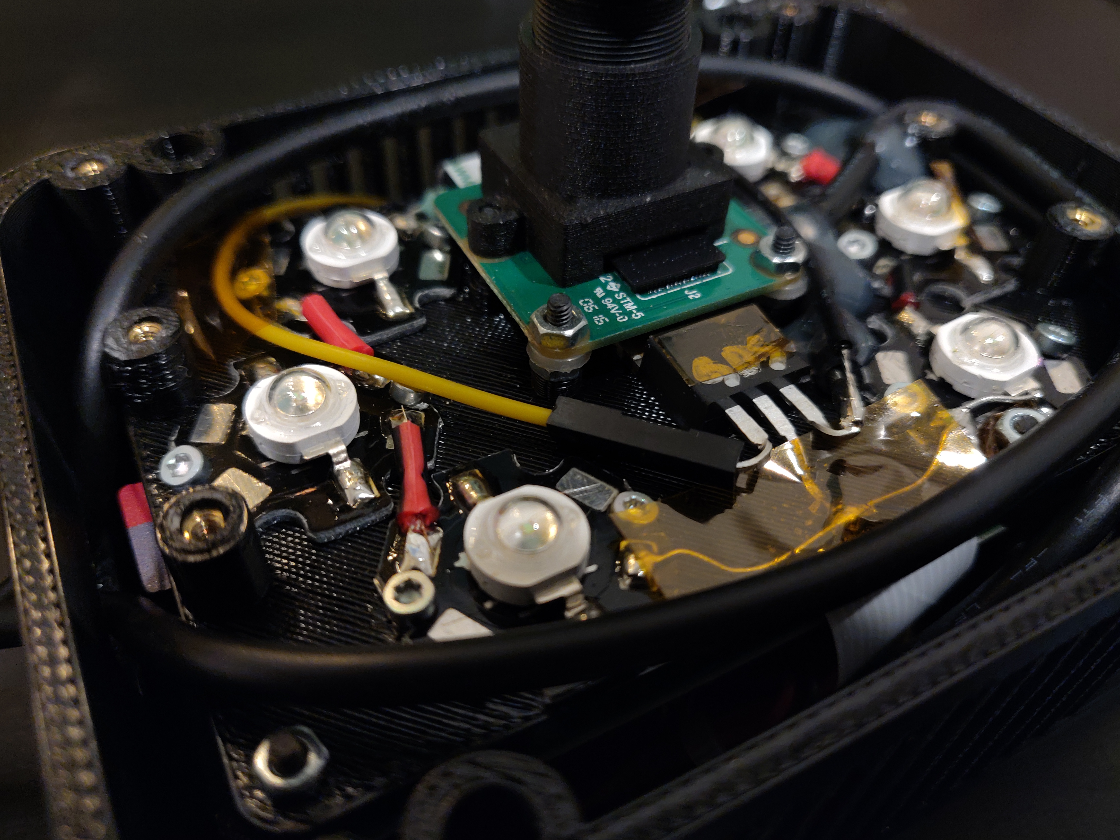
This used an overclocked Raspberry Pi 4, which was significantly faster than the Pi 2, had 6 high-power LED's that shone 600 lumens bright, a lens mount for the camera, and a proper case to hold it all together. It finally provided for an easy way to handle the hardware and met all the requirements we needed, compute and otherwise.
Challenges
A lot. One of the biggest issues was performance. This needed to run on a compact platform so I couldn't just throw bigger, more powerful hardware at it. This forced me to be diligent about the code I wrote, making sure it was as efficient as I could make it. I also learned how to profile my code and log events so I could analyze which parts were the most computationally expensive.
Another thing was the hardware. I'm a programmer first, so learning to CAD and doing the electrical work was definitely a (fun) challenge for me. Particularly because this demanded a lot in a very small form factor, so as I was trying to figure out how to fit these individual components together, I also had to consider power delivery and cooling.
What I Learned
A lot. I learned about web servers, WebSockets, threading (how threading on Python is different from other programming languages), multiprocessing, inter-process communication (IPC) via pipes, queues, stacks, and sockets, double buffering, a lot of OpenCV, how to profile my code, and how to write efficient code. I also learned a bit of SolidWorks, some new things about electronics, and how to use tools like multimeters and calipers.
Something else I learned was how to design and implement a system as intricate as this was. Most of my time was spent doing research and planning. For example, when I needed to parallelize the software for better performance, I researched how multiprocessing works, the different methods of IPC and when each should be used. From there I would plan out by hand on paper what I needed to implement. For example, how many threads/processes I'd need, what each thread/process was responsible for, the lines of communication between them and what they were communicating to each other. This in-depth research and planning was crucial as it lead to a better design and it made implementation much smoother. This process also served as a form of documentation for my project, which made future modifications/additions easier to perform.